The A3 Interval Test Method

The A3 Interval Test Method – What is it?

The A3 Interval Test Method (Method A3) is a calibration interval optimization algorithm that employs accumulated calibration history for a given item(s), make/model, or similarly classed instrumentation (e.g. all 3½ digit handheld digital multimeters, or all 1% FS pressure gauges) to test statistically whether the subject’s assigned interval is appropriate.

The result of the test determines whether to adjust the current interval, or not, based on calibration results consistent with End of Period Reliability (EOPR) expectations.

For example, if the calibration laboratory has an EOPR target of 89%, the algorithm will perform a statistical analysis on the selected item(s), make/model, or class and recommend one of 3 possible actions:

1. Extend the current interval – the subject analyzed is performing above expectations therefore less frequent calibrations are required.
2. Take no action - the subject analyzed is performing as expected therefore no remedial action is required.
3. Reduce the current interval - the subject analyzed is performing below expectations therefore more frequent calibrations are required.

How does it work?

The Method A3 algorithm is based on statistically significant results in lieu of a reactionary method.

A reactionary method is a simple algorithmic method that does not utilize any statistics. An example of a reactionary method (common in many labs) is outlined in the steps below:

1. Last 3 calibrations in-tolerance?
   1. Yes = lengthen the current interval by 1.5x (or extend by 10-15% of the current interval)
   2. No = decrease the current interval by 0.5x

Utilizing a reactive method applies no statistical reasoning in deciding the outcome. The end user is responding to random occurrences. This results in many wrong decisions to extend/decrease a calibration interval.

Another flaw in using reactionary methods is target reliability accuracy. Simulations indicate the time taken to settle on “a” given interval can take anywhere from 10 to 60 years. Even if a “settled” point emerges, there is no indication it settled on the correct interval. It can ultimately settle on an incorrect interval, and it will not respond to any further data regardless of observed reliability.

How Method A3 differs from algorithmic responses is by utilizing statistical significance. What is meant by statistical significance “is my current interval correct?”

The example above estimates the EOPR by simple division, which provides “a” number but disguises the confidence associated (it is not “the” number). For example, if a particular make/model instrument were calibrated 10 times with no “Out Of Tolerance” (OOT) noted, using simple math we discover the EOPR is 100%. The problem with this simplistic approach is in the event of zero failures, the EOPR appears to be 100%, which is incorrect as virtually nothing could possibly be 100% reliable, uncertainty is always an unseen variable.

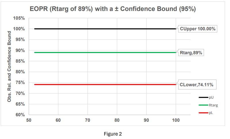
Although 10 out of 10 items were found “In-Tolerance”, the true reliability is somewhere between the reliability confidence bounds. If the servicing lab has an EOPR target of 89% with 95% confidence, and zero failures, the worst-case EOPR is assumed to be the lower calculated confidence bound, which is 74.11%. In the manufacturing realm, this is known as a Receiver Operator Curve (ROC).

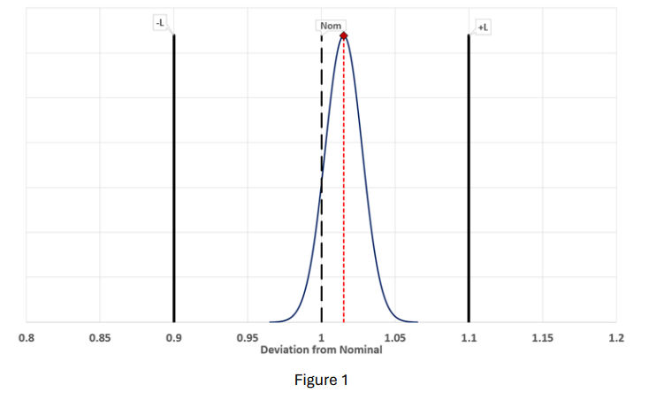
Think of EOPR the same way we think about a nominal value and a surrounding ± tolerance. For example, we have a nominal value of 1 VDC with a tolerance of 1.1 to 0.9 VDC at 95% confidence. One would never make a measurement, say 1.015 VDC, and consider it a valid measurement if no tolerance information and/or the uncertainty was not provided. EOPR works in a similar way.

Taking the voltage example, the value of 1 VDC is bound by 0.9 to 1.1 VDC. If the measured value is +1.015 VDC, the measurement is considered “In-Tolerance.” The true value, however, is unknown. It is unknown because of the measurement uncertainty involved. The true value lies within the measured value and the associated uncertainty. This is the case for any measurement situation as uncertainty is unavoidable.

By using the substituting binomial functions as a tolerance bound concerning the reliability, the similarity between acceptance/rejection criteria becomes obvious. Instead of the deviation from nominal, the question now becomes “is the reliability in tolerance?”

By taking figure 1, flipping it 90º horizontally, and substituting binomial confidence bounds, the example of 10 calibrations with 10 successes now places a “tolerance” around the EOPR target (Rtarg).

Since the green line (Rtarg of 89%) is between the upper calculated binomial limit (CUpper 100%) and the lower calculated binomial limit (CLower 74.11%), the algorithm makes no suggestion to increase/decrease the current calibration interval because both the EOPR (Rtarg 89%) and the confidence 95% are within “spec” (figure 2).

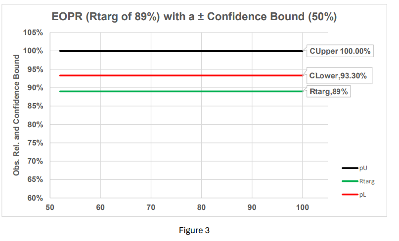
It should be noted, the ± binomial limits are not static entities, they widen/narrow with respect to accumulated data (sample size) and confidence levels.

Keeping the same resolution on the graphic (figure 3) and changing only the confidence from 95% to 50% narrows the “tolerance” around the EOPR. Also, since the lower binomial (CLower 93.3%) is above the EOPR (Rtarg 89%), the algorithm will suggest increasing the interval. It should be noted that changing confidence from 95% to 50% means you are 50% certain you are making the correct choice.

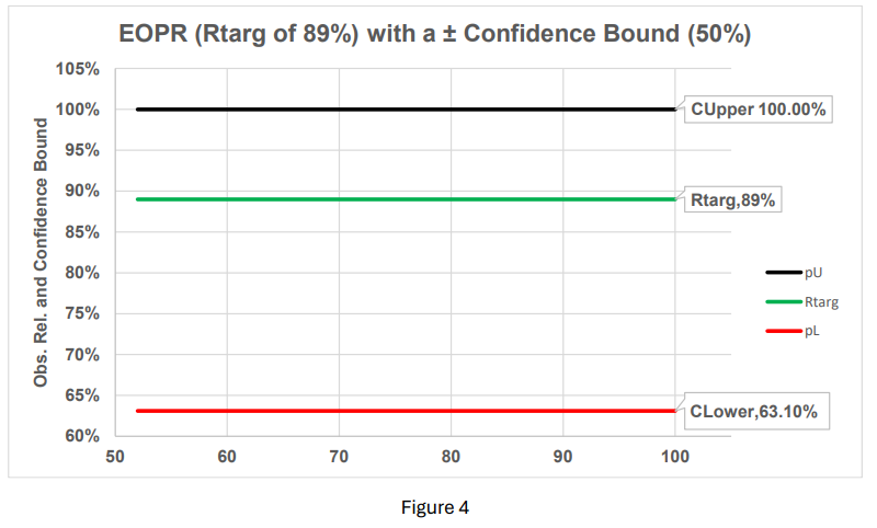
Consequently, changing only the confidence from 50% to 99% widens the “tolerance” offering no reason to change the current interval (figure 4).

Desiring a high reliability target, coupled with high confidence, does not mean bigger is better. In fact, it carries unreasonable sample sizes and likely will negate the reason for using interval analysis altogether. For example, if the end user required an EOPR of 99.9%, coupled with 99% confidence about that reliability target, a total of 4,603 calibrations would need to be recorded, **** , just to demonstrate that level of certainty. It’s likely the assets tested would be scrapped before the end target goal appears.

The basic algorithm

When using this program, an interval is “tested” to determine if it is at the correct interval. If the interval tested is 365 days (as an example), you must set some default acceptance criteria. A recommendation, for 365 days, is excluding any calculated interval that is outside the hard interval of 365 days by ~16.4% (a calculated interval is current cal date – previous cal date). Why 16.4%?

The case for a percentage of 16.4% is because customers may turn in their equipment earlier than the scheduled due date or the customer may turn in the equipment delinquently (either due to a requested interval extension of 30 days + the due date, or simply delinquent). This results in ± 60 days (your criteria may vary). The program will gather all calibration statistics, rejecting any calculated actual intervals that are outside the hard interval of 365 ± 60 days.

Setting a reliability target

A reasonable compromise is an EOPR target of 89% coupled with 95% confidence. These values are not arbitrarily selected. There is a solid reason for this combination. The EOPR is a key component to utilizing measurement decision risk (aka guard-banding). Many organizations adhere to providing conformance testing results that have a 2% or less Probability of Fale Accept (PFA). Although outside the scope of this documentation, maintaining both the UUT and the reference standards at 89% EOPR ensures no matter the Test Uncertainty Ratio (TUR), the PFA will never exceed 2% PFA (1.95% is maximum per figure 5). This was first documented by Scott Mimbs in 2011 as a response to meeting ANSI Z540.3 2% PFA rule. Method A3 helps achieve this goal.

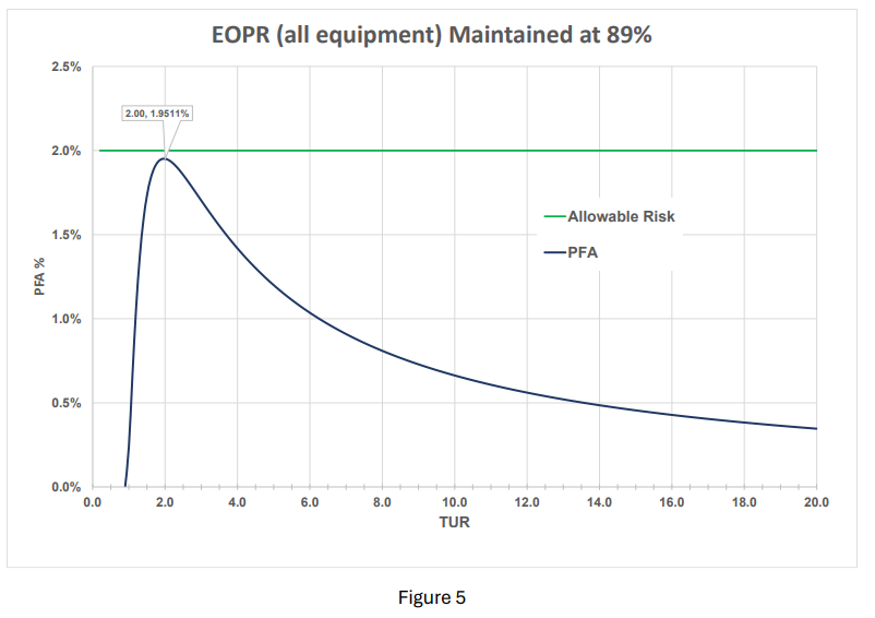
The reader may be asking themselves “why, if TUR is decreasing, does the PFA peak then fall?” The reason for this phenomenon is once the maximum PFA is reached, with the diminishing TUR, the probability of falsely accepting a bad product (or process) decreases sharply and virtually any product (or process) tested will be falsely rejected instead of falsely accepted.

Why should I use it?

The utilization of calibration interval analysis isn’t simply for maintaining reliability targets and minimizing PFA considerations, it is a very real metric driver allowing any organization to make informed decisions about their current inventory Operational & Maintenance (O&M) budgets as well.

NOTE: To fully exploit the benefits of this feature, it would benefit the organization to establish standard hours (per calibration type) and the internal loaded costs associated with the tasking.

Referencing the beginning of this document, it was pointed out three basic outcomes result by using an optimization program.

1. Extend the current interval – the subject analyzed is performing expectations therefore less frequent calibrations are required.
2. Take no action - the subject analyzed is performing as expected therefore no remedial action is required.
3. Reduce the current interval - the subject analyzed is performing expectations therefore more frequent calibrations are required.

When it comes to O&M budgets and changing the scheduled intervals, we like to call these: good news, no news, and bad news. We will look at #1 and #3 specifically as #2 requires no action.

Example: First, the good news. Let’s assume for a specific make/model you have 1000 total calibrations. This is not necessarily on a single item but rather on a group of the same (or similar) make/model. Keeping the EOPR and confidence levels at stock settings (89% EOPR and 95% confidence), and assuming the data passed the criteria, the calibration interval is increased from 365 days to 438 days (+20%).

If the time to calibrate each item is 1.5 hours, and the internal loaded cost (pension & benefits) is $150/hr., and there are 1000 of these like items in your inventory, the current O&M budget for this single make/model is ~$225,000. The output result is 1000 x 1.5 (hours) x 150 (dollars) = $225,000.

We know the savings are 20% from our previous calculations, therefore $225,000 x 0.2 = $45,000.

Now the bad news. Let’s assume that another make/model is performing poorly and needs the interval shortened (all criteria is the same for reliability) from 365 days to 257 days (~30% reduction). We have 500, ± 1% pressure gauges not meeting the reliability target. These items take 1.0 hours to calibrate. Now we have 500 x 1.0 (hours) x 150 (dollars) = $75,000. But instead of calibrating these items annually, they must now be every 257 days due to our finding. This essentially increases the O&M cost from $75,000 to $97,500 (+30%).

Now the bottom line: Original cost for the 2 make/models = $300,000 per year.

Item 1 now = $180,000 per year O&M

Item 2 now = $97,500 per year O&M

Total cost = $227,500

Net savings = $300,000 - $227,500 = $22,500

The question now becomes, “why wouldn’t you use it?”